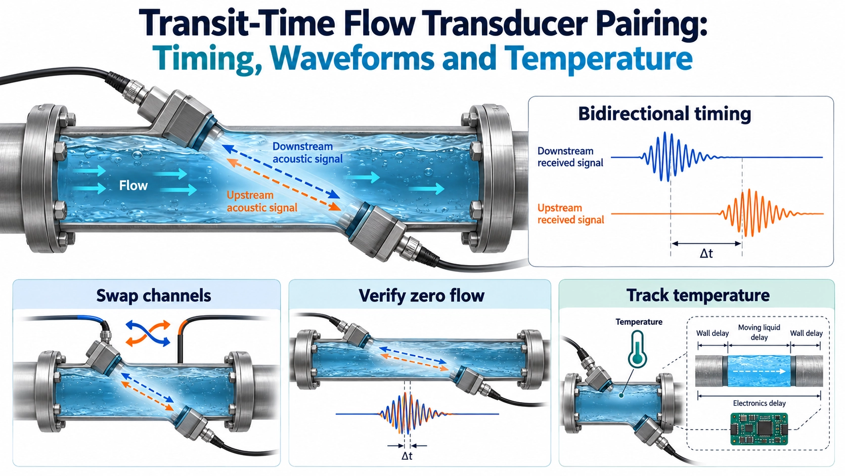
The useful question is whether the pair preserves the time difference
Two liquid-flow transducers can have similar resonance curves and still produce an unwanted zero-flow offset in a finished measurement channel. Conversely, slightly different received amplitudes do not automatically make a pair unusable. For transit-time flow measurement, the decision is whether the complete upstream and downstream acquisitions deliver a stable, interpretable propagation-time difference over the intended operating conditions.
This is an OEM pairing problem, not a general incoming-inspection tutorial. It involves two transducers, their mounting, the liquid path, cables, transmit/receive switching, gain and the time estimator. A pair should therefore be evaluated with a defined measurement strategy. Recording only two nominal frequencies or one room-temperature signal amplitude leaves the most important question unanswered.
Separate fluid transit time from the measured system delay
For an ideal straight acoustic path of length L in a uniformly moving fluid, let c be sound speed and v the axial flow velocity. If the path makes an angle θ with the flow axis, the fluid-only times are:
tdown = L / (c + v cos θ); tup = L / (c – v cos θ).
For flow velocity small relative to sound speed, the difference is approximately Δt = tup – tdown ≈ 2Lv cos θ / c². These expressions explain why a small directional timing difference matters. They are not a complete calibration equation for a real flow channel. Wedges, pipe walls, matching layers and electronics can add delay; they must not simply be treated as part of the moving-fluid path L.
The comparison of transit-time and Doppler flow measurement covers the underlying method choice. Here the focus is narrower: identifying which part of the difference belongs to flow and which part comes from directional asymmetry or changing test conditions. Common delay and differential delay have different consequences; total travel time alone cannot separate them.
Look at both waveforms before reducing them to two numbers
The BBFM-Q1M liquid-flow transducer has configurations operating around 1 MHz for flow-metering integration. Its mechanical, bandwidth and electrical options should be selected as coherent configurations, not mixed into one assumed specification. The product is an acoustic component; selecting two units does not by itself establish a matched set for every circuit or guarantee a completed meter’s accuracy.
Acquire the actual terminal excitation and the received signal in both directions. Fix burst settings, polarity convention, gain, filtering and the estimation window, or explicitly log any directional differences. Compare envelope, early arrivals, useful cycles, ringing, clipping and noise. A larger peak is not necessarily a better timing signal if it arrives with saturation or a distorted leading section.
Different estimators respond differently to waveform changes. An amplitude threshold can move its crossing when amplitude changes. Correlation can be robust, but still select the wrong cycle or respond to a changed window. At 1 MHz, one cycle lasts 1 µs: a cycle-selection mistake must not be treated as ordinary small timing scatter. Preserve raw waveforms and estimator diagnostics so that a plausible-looking final flow value does not hide the error.
Use controlled changes to locate the asymmetry
| Comparison | What stays controlled | What the result helps identify |
|---|---|---|
| Reverse transmission direction | Same assembled path, liquid state and documented settings. | Directional amplitude, waveform and timing differences. |
| Exchange electrical channels | Keep transducers and mechanical mounting unchanged where feasible. | Effects associated with switching, gain, sampling or cable routing. |
| Exchange transducer positions | Re-establish the same mounting and acoustic geometry. | Interactions that follow a component or a mounting position. |
| Repeat after reconnecting or reassembling | Use a defined assembly procedure and the same estimator. | Whether apparent pairing depends on an unstable connection or coupling. |
| Repeat across temperature conditions | Record liquid, fixture and electronics temperatures and settling state. | Common drift, differential drift and sensitivity to gradients. |
Make one change at a time. If a difference follows a transducer, that identifies an interaction worth investigating; it does not prove a defective ceramic element. Source and receiver impedances, cable loading and mounting can make a nominally reciprocal acoustic path appear different through the complete electronics. If a difference follows a channel, investigate that channel before rejecting the transducers.
Modern measurement electronics combine pulse generation, analogue interfaces, gain and sampling. The Texas Instruments MSP430FR6047 ultrasonic-sensing documentation illustrates those separate functions. This is background for defining a test boundary, not a requirement to use that device or a transfer of its published performance to BBFM-Q1M.
Prove the zero-flow condition, then examine temperature
Stopping a pump is not sufficient evidence of zero flow. Residual circulation, thermal convection, leakage or changing pressure can remain. Document how the test loop establishes a stable reference condition, and interleave upstream and downstream measurements closely enough to avoid interpreting changing liquid conditions as a directional difference. State the acquisition sequence and its timing.
At each condition, record the signed upstream-minus-downstream result, its mean, variation and repeatability after restart. Do not report only an absolute difference or an average that conceals sign changes. A stable offset and a fluctuating offset create different calibration problems. Retain both fluid transit-time estimates as well as their difference; a common shift can otherwise be invisible in the reported Δt.
Test uniform temperature changes separately from temperature gradients. A fixture that has reached equilibrium does not represent one transducer being heated while the other remains cool. Record temperatures at meaningful locations and allow adequate settling before assigning a steady-state result. Include the cables and electronics relevant to the operating installation: temperature effects are not restricted to the piezoelectric material.
Repeat in the finished channel when changing seals, preload, adhesive, housing or cable arrangement. Bench pairing in water is evidence for that fixture, not automatic proof of the final flow tube. Any zero correction must be checked across temperature and assembly states; it should not be used to conceal wrong-cycle selection or unstable coupling.
Define acceptance from the low-flow requirement
There is no universal nanosecond pairing tolerance for all 1 MHz transducers. Derive the allowable residual timing error from the instrument’s low-flow objective, actual path geometry, estimator and uncertainty budget. Then allocate what can be contributed by components, mounting, electronics and compensation. The general transducer testing guide supports the underlying component checks; the additional deliverable here is a paired, bidirectional flow-channel record.
- Identify both components, their exact configurations, positions, cables and test electronics.
- Keep bidirectional waveforms, timing settings, estimator version and signed results together.
- State how zero flow, thermal equilibrium and representative gradients were established.
- Report repeatability after reconnection or assembly, not only the best initial trace.
- Verify complete flow measurements against an appropriate reference at relevant flows and temperatures.
For a pairing discussion with Deep Minds Ultrasonic, provide the flow-channel drawing, liquid and temperature range, expected low-flow performance, burst and acquisition settings, and the proposed acceptance method. Define how replacement units will enter an existing pair. The result should be a reproducible integration specification, with component pairing clearly separated from full-meter calibration and regulatory approval.